Error #VALUE! in Excel

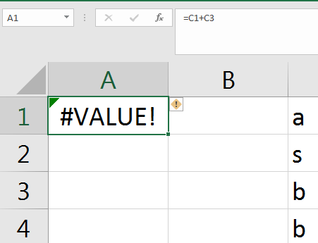
One of the common error Microsoft Excel error is VALUE!. This error occurs when your formula has the wrong type of argument (i.e., a mix of text and numeric fields). You can fix this error if you use functions instead of operators & check that you’re referencing the correct cells.

Error #NAME? in Excel

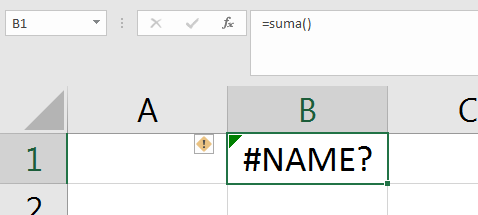
One of the common error Microsoft Excel error is #NAME?. This error occurs when Excel doesn’t recognize text in a formula. You can fix this error if you ensure your formulas are typed correctly, and that any text is enclosed in quotation marks. For example, if you are trying to place a formula in Spanish in a version of Microsoft Excel that is in English will give the error #NAME?.

How to Protect cells in Microsoft Excel

We are going to study the protection of cells available in Excel so as not to allow the modification of cells by mistake or by not having permission to do so.

Protect cells

In addition to password protection for workbooks, Excel offers several orders to protect the cells of the workbook. For this we have to perform two operations: the first consisting of protecting the cells that we don’t want to suffer variations, and the second consisting of protecting the sheet.

When a cell is blocked it can’t suffer variations. Actually by default all the cells are protected or blocked so that they do not suffer changes, but we do not realize because the sheet is not protected, so that the cells are actually blocked before the spreadsheet has to be protected.

To unblock the cells that we want to vary at some point, follow these steps:

Select the range of cells that we want to unblock to make variations.

Select the menu Home → Format.

Choose the option Format Cells…

Click on the Protection tab. The following window will appear:

Deactivate the Locked box and click on the OK button.

If the Hidden box is activated, what is intended is that the formula or the value of the cell can’t be displayed in the formula bar.

The operations of the Protect tab have no effect if we don’t protect the spreadsheet, therefore we will have to carry out the following steps:

Select the menu Home → Format.

Select the option Protect sheet…

The Protect Sheet dialog box appears:

Leave the box Protect worksheet and content of locked cells activated to protect the contents of the cells in the active sheet.

Activate the desired options in the Allow users of this worksheet to box, so that the protection for the selected modification has no effect and deactivate it to take protection into account.

If we want to assign a password so that only the person who knows the password can check out the sheet, write it in the Password box.

Click on the OK button.

If we have entered a password, it will ask for password confirmation, therefore, we will have to retype it and click on the OK button.

From now on, the active sheet is protected, so it will not be possible to modify those cells that were blocked at first.

If we want to unprotect the sheet, we will perform the same steps as in the protection, that is:

Select the menu Home → Format.

Select the option Unprotect sheet…

If we had assigned a password, it will ask for it, so we will have to write it and click on the OK button. If there was no password assigned, it automatically checks it out.

If you need help with data, schedules, plans and budgets, do not hesitate to contact me.
Uses of Excel for teachers

Excel is a versatile program that can be used in many areas. One of the areas where it is most useful is in education. Then I explain the 5 uses of Excel in the educational area.

School grades

You can keep track of your students’ grades, and without much effort, take the average of grades, percentages and totals at the end of the year.

Graphics

You can track your students’ grades in a visual way through graphics.

Lists of students

You can also keep track of the students you have, their important data and their history.

Lists of teachers

You can keep track of the teachers, their general data, and other relevant information.

Schedule

You can keep an agenda with evaluation dates, events and others in an easy way.

If you need help with data, schedules, plans and budgets, do not hesitate to contact me.

What is Excel and what is it for?

Excel is a spreadsheet integrated in Microsoft Office. This means that if you already know another Office program, such as Word, Access, Outlook or PowerPoint, you will be familiar with using Excel, since many icons and commands work in a similar way in all Office programs.

It probably does not help much to know that Excel is a spreadsheet, do not worry, now I’ll explain it to you. A spreadsheet is a program that is able to work with numbers in a simple and intuitive way. To do this, a grid is used where numbers, letters and graphics can be entered in each cell of the grid.

For example, to add a series of numbers you just have to enter one below the other, as you would do on a piece of paper, place yourself in the cell where the result will go and tell Excel that you want to make the sum of what you have on top.

You may think that to make a sum it is better to use a calculator. But think about what happens if you make a mistake entering a number in a sum of 20 numbers, you have to re-enter all of them; While in Excel it does not matter if you make a mistake when entering a data, you simply correct the data and Excel automatically calculates everything again.

This is important when the calculations are a little more complicated, imagine you are making the income statement by hand and in the end you discover an error, you would have to re-calculate everything. If you do it with Excel you only have to correct one data.

This automatic recalculation feature also allows you to make simulations easily. For example, if you are calculating what you will have to pay per month when applying for a mortgage loan, it is sufficient that you enter different amounts in the amount of the loan so that you can see what you would have to pay in each case.

For more information and help with your spreadsheets in excel or to migrate from excel to a robust web system with databases do not hesitate to send me an email.

How to create dependent drop-down lists in Excel

Many times we have to make some drop-down list in Excel and that these are dependent on another list. Here I will show you how to create them in an easy and simple way.

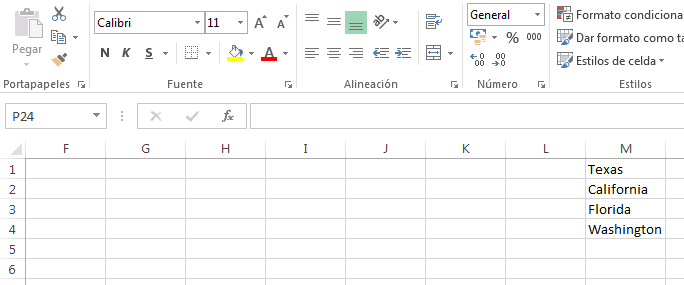
  • We create a macro list on which the second drop-down list will depend. In our example, they are States of the United States.
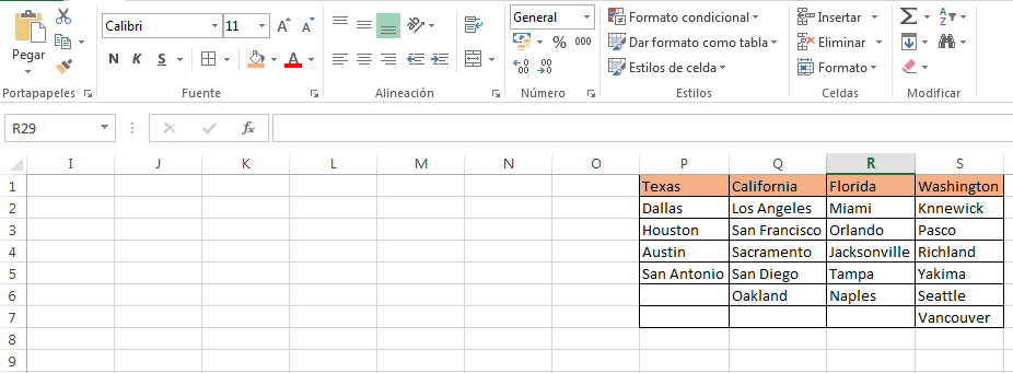
  • Then we create the list that will be dependent on the first one. In our example it will be the cities of the states that we have selected.
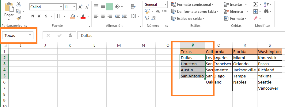
  • We select the first range of cities, in our example the cities of Texas and we put a name in the name box that appears on the upper left side, where we usually see the cell number. It is important that the name does not contain spaces, accents or special characters, and that it is exactly the name that we have placed in the name of the state. Then we click on enter.
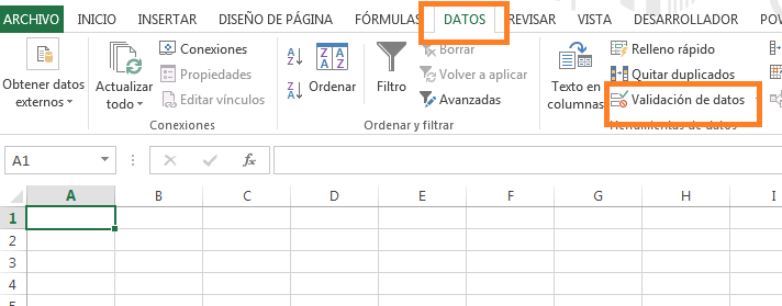
  • Now let’s create the drop-down lists. We select where we want the first drop-down list to appear and go to the Data -> Data Validation menu.
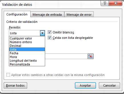
  • In the window that appears, select Allow -> List.
  • In origin we select the cells where our macro list is, in our example the states.
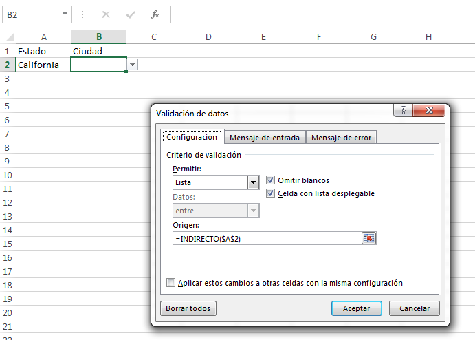
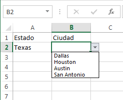
  • With this we would have the first drop-down list. To create the drop-down list of cities dependent on the states, we again select the cell where we want the cities to be and go to the menu Data -> data validation, select in Allow -> List, and in origin we will place the function “= INDIRECT ( $ A $ 2) “. Inside the parenthesis we will place the cell where the dropdown of the macro list is, in the example in cell A2.
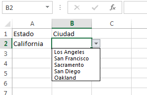
  • Finally we have a list of the city depending on the state that we select.

If you have problems with your spreadsheets in excel I can help you, just send us an email with your questions or project. I’m to order.

Fiverr